Trust on the Line:

To achieve business goals, your plans must account for the impact of material Cybersecurity events—such as data breaches, ransomware, and extortion—on the business’ ability to execute its strategy. A systematic approach is essential for understanding and preparing for these events, ensuring the business can respond effectively and create the conditions needed to succeed and thrive, even in the face of cyber incidents.

Beyond your business’ resilience to Cybersecurity events and the immediate costs of incident response, a critical factor in long-term success is the damage to your brand, reputation, and customer trust. These factors hinder growth by creating headwinds for new sales and reducing revenue, as existing customers down-sell or churn in response to diminished trust.

This article tackles the problem of calculating the financial impact of material Cybersecurity events in order to inform risk mitigation and enable strategic decision making.

Why Model the Fallout of Reputation Risks on Financial Outlook?

The long-term impact of Cybersecurity incidents on customer trust and brand perception can erode a company’s market position and growth potential. Thus, modeling these risks allows businesses to quantify potential losses, giving leaders a clearer picture of how incidents could affect key financial metrics like revenue, down-sell, and churn. Armed with this data-driven insight, organizations can make informed decisions about risk management, investment in cybersecurity, and strategies for mitigating the downstream effects of security breaches on trust and revenue. By proactively understanding these risks, businesses can better protect their growth and ensure long-term business resilience.

The Economics of Trust and Reputation

Several studies have shown that Trust and Reputation can have significant material effect on a company’s profitability. For example, research carried out by Accenture shows that trust has “material” effect on a company’s bottom line. In their global risk management survey, Aon also identified reputation risk caused by reputation events, such as cyberattacks, as a formidable factor that can have a material impact on shareholder value and the cost of capital post-event. This phenomenon applies to companies of different shapes and sizes and across different verticals to different degrees. This article will focus on Software as a Service (SaaS) companies as the archetypal example, although the principles discussed are applicable to various business models.

When customers decide whether to purchase a company’s products or services—and whether to remain loyal in the face of competition—trust and reputation play a crucial role. If these are compromised, companies face increased down-sell, customer churn, and ultimately, lost revenue and reduced long-term profitability.

Supporting Decision-Making

Our goal is to enhance strategic decision-making by quantifying the impact of cyber events on trust and, ultimately, on essential financial metrics. Understanding this relationship enables your organization to anticipate and mitigate potential financial risks. The types of questions we aim to answer include:

What is the likelihood of down-sell and churn exceeding a specified threshold?
What are the chances that new annual recurring revenue (ARR) will meet or exceed targets despite cybersecurity incidents?

Answering these questions involves calculating exceedance probabilities—which indicate the likelihood that financial metrics, such as down-sell, churn, or new ARR, will meet or exceed defined thresholds.

To calculate these probabilities, we construct exceedance curves for key financial metrics based on a trust model and Monte Carlo simulation data. (Loss) Exceedance Curves are commonly used to communicate the probability of exceeding specific loss magnitudes, serving as a standard tool in cyber risk assessment frameworks like FAIR.

Below is an example of exceedance curves for down-sell and churn (D&C) and new ARR due to trust-impacting cybersecurity events. With these curves, we can answer questions such as: “What are the chances of down-sell and churn exceeding $1 million due to material cybersecurity incidents?”

ARR and D&C exceedance

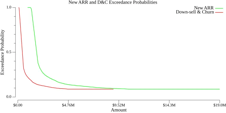
By analyzing the exceedance curves, decision-makers gain valuable insights into the probability of down-sell and churn reaching concerning levels in the aftermath of material cybersecurity events. This approach also helps assess the likelihood of not meeting ARR growth targets, which can influence long-term strategies.

Armed with this information, leaders can make more informed decisions on risk tolerance, mitigation strategies, and resource allocation to reduce the likelihood, severity, or duration of trust-impacting cybersecurity events.

With these objectives in mind, let us now explore how to derive these metrics through trust and reputation modeling combined with Monte Carlo simulations.

Modeling Trust and Reputation

Trust and brand reputation are built over time but can be quickly damaged by significant cybersecurity events, especially if these incidents occur frequently and in quick succession.

We can model trust and reputation ( $\Tau$ ) as a continuous function of time, ranging from 0% (no trust) to 100% (maximum trust and reputation), as follows:

Trust and Reputation Model

\Tau(t,i) = 1-e^{-k(t-t^i_0)}

where:

$t$ is time, measured in days
$k$ is a trust and reputation growth factor for your organization
$t^i_0$ is a trust erosion level after the trust-eroding incident $i$

The growth factor, $k$ , varies depending on your organization’s ability to build and restore trust over time. It is influenced by factors such as brand strength, product quality, and response effectiveness following a reputation-impacting event. In this model, $k$ is left as a parameter you can set to reflect your organization’s specific characteristics.

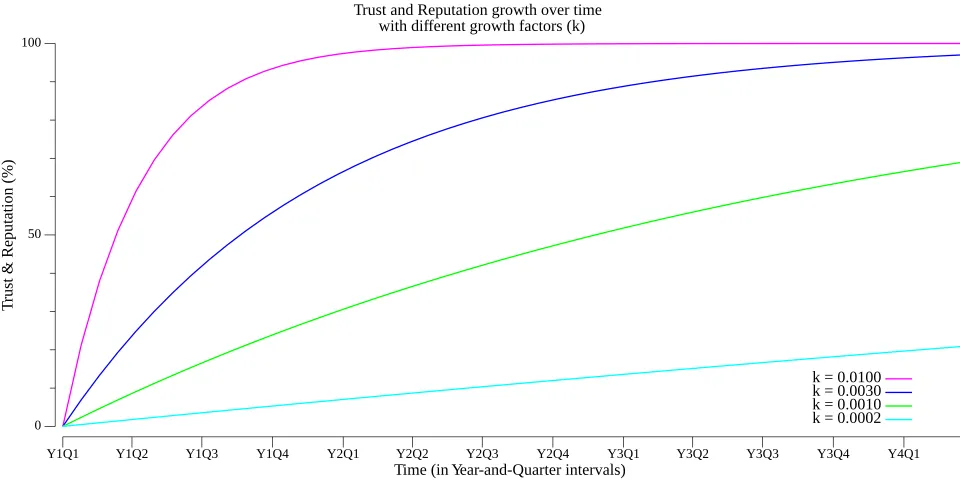
The graph below demonstrates how trust and reputation grow over time, starting from an initial “Genesis” point, such as Year 1, Quarter 1 (Y1Q1), based on an appropriate growth factor $k$ .

Trust and Reputation modeling

Modeling the Trust Impact of a Loss Event

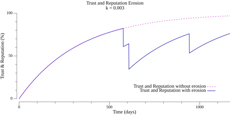
When a reputation-impacting loss event—such as a cybersecurity breach or major outage—occurs, there is a corresponding reduction in trust and reputation. The graph below illustrates how three such events lead to a decline in trust over time (the blue plot). In this example, the trust growth rate $k=0.003$ , and the company experienced three incidents on days 577, 608, and 943. The red dotted line represents the growth trajectory without any trust-eroding events.

Trust Depletion

For those seeking guidance on how to model trust fluctuations in the presence of such events, an example is provided below.

Trust Erosion Modeling

click to open/close

Below, we demonstrate how to model the erosion of trust and reputation following a material event.

We consider three factors as drivers of trust erosion:

The Loss Magnitude ( $M_i$ ) of event $i$ , which reflects the severity of the event and the level of public exposure
The Time Since Last Event ( $t_i - t_{i-1}$ ), which captures how close together successive material events occur.
The Recovery Time (TTL $_i$ ), which measures how long it took to recover from the event $i$ and restore normal services.

Trust and Reputation After Loss Event

\begin{align} \Tau(t,i) &= 1- e^{-k(t - t^i_0)} \nonumber\\ \nonumber\\ t^i_0 &= -\dfrac{1}{k}\ln\left(1- T(t^+_i)\right) \nonumber \\ \Tau(t_i^+) &= \alpha_i \times \Tau(t_i^-) \nonumber \\ \alpha_i &= 1- \left(w_m \times \dfrac{M_i}{M_i + \tau_m} + w_\Delta \times \dfrac{\tau_\Delta}{(t_i - t_{i-1}) + \tau_\Delta} + w_{\text{TTL}} \times \dfrac{\text{TTL}_i}{\text{TTL}_i + \tau_{\text{TTL}}} \right) \nonumber \end{align}

where:

$t_i$ is the time the loss event $i$ occurred, and $t_{i-1}$ is the time of the previous event
$\Tau(t_i^+)$ is the trust and reputation level immediately after event $i$
$\Tau(t_i^-)$ is the trust and reputation level immediately before event $i$
$\tau_m$ is the loss magnitude tolerance factor
$\tau_\Delta$ is the time between events tolerance factor
$\tau_{\text{TTL}}$ is the recovery time tolerance factor
$w_m, w_\Delta$ , and $w_{\text{TTL}}$ are the weights for loss magnitude, time since last event, and recovery time, respectively.

Predicting the Effect on the Bottom Line

To understand how material events affect critical business metrics, we focus on Down-sell and Churn (D&C) and New Annual Recurring Revenue (ARR). The approach to modeling this impact is summarized below.

Predicting Business Impact by Simulation

Trust and Reputation ( $\Tau$ ) is modeled to decline with events and gradually recover over time, asymptotically approaching 1.
D&C and New ARR are influenced by $\Tau$ , where higher trust results in lower churn and improved growth.
Use Monte Carlo simulations to generate event scenarios, model trust evolution, and estimate D&C and New ARR.
You can take the analysis further by applying Bayesian updates to refine the parameters of the model based on observed data (e.g. from sales and marketing), improving future predictions.

We have already introduced a model that represents Trust and Reputation over time, factoring in trust-eroding events.

Lagging indicators

Before defining our model further, it’s important to consider that the variations in New ARR and D&C should and could be designed as lagging indicators of trust evolution, factoring in other operational elements like contract expiration terms and sales cycles.

While we won’t go into extensive detail here, it’s useful to note that there is a natural delay to the onset of D&C following a significant event, allowing time for the effect of damaged trust to propagate through contract renewal processes. However, if your analysis is over a longer time horizon, e.g. 3 years, that delay nuance may not matter.

Trust Impact on New ARR and D&C

Now, let’s define how D&C and New ARR depend on Trust, time, and trust-eroding incidents.

A Model of ARR and D&C

\begin{align} \text{ARR}(t,i) &= \text{ARR}_0 \times \alpha(t,i) \times \Tau(t,i) \nonumber \\ \text{DC}(t,i) &= \text{DC}_0 \times \beta(t,i) \times (1 - \Tau(t,i)) \nonumber \\ \end{align}

where:

ARR $(t,i)$ : New ARR over time after the material event $i$ .
ARR $_0$ : Baseline growth factor for new ARR in the absence of material incidents.
DC $(t,i)$ : Down-sell and churn over time after the material event $i$ .
DC $_0$ : Baseline down-sell and churn rate without material incidents.
$\alpha(t,i)$ and $\beta(t,i)$ : Time-dynamic trust sensitivity factors for ARR and D&C, respectively.

The time-dynamic trust sensitivity factors, denoted as $\alpha(t,i)$ and $\beta(t,i)$ , help fine-tune how ARR and D&C metrics respond to changes in trust over time. These factors can be defined as simple constant scaling terms, or they can incorporate more advanced time-dependent dynamics to capture nuanced effects such as time delays and variable sensitivity to trust fluctuations.

Below, we outline a potential approach for defining these factors, along with additional considerations for incorporating more complex dynamics.

Defining Time-Dynamic Sensitivity

click to open/close

Below is a possible definition for $\alpha(t,i)$ and $\beta(t,i)$ :

Time-dynamic sensitivity factors

\begin{align} \alpha(t,i) &= \alpha_0 + \alpha_1e^{-c_\alpha(t-t_i)} \nonumber\\ \beta(t,i) &= \beta_0 + \beta_1e^{-c_\beta(t-t_i)} \nonumber\\ \end{align}

where:

$\alpha(t,i)$ and $\beta(t,i)$ : Time-dynamic sensitivity factors for ARR and D&C, respectively.
$\alpha_0,\alpha_1, c_\alpha, \beta_0, \beta_1, c_\beta$ : Constants that adjust the sensitivity. This, for example, allows sensitivity to be higher immediately after an event and to decay over time, capturing both the short-term impact and gradual diminishing effect of the events.

If you’re curious about why we defined $\alpha(t,i)$ and $\beta(t,i)$ as we did, or if you’re questioning why the ARR and D&C sensitivities shouldn’t have a straightforward linear relationship with trust, see the additional considerations below.

Additional Considerations for New ARR and D&C Sensitivities

It might seem intuitive to assume that ARR and D&C should be directly and linearly correlated with trust and reputation, without requiring additional dynamic sensitivity to time and material events. After all, the trust model already accounts for time and the impact of such events. However, there are important reasons why we introduced dynamic sensitivity factors in our model, and the following considerations will help clarify the motivation behind this approach.

Key Justifications for Dynamic Sensitivity Factors ( $\alpha(t,i)$ and $\beta(t,i)$ ):

Decoupling Trust and Financial Impact
- Trust and reputation ( $\Tau$ ) measure an internal factor—how customers perceive the service provider. On the other hand, financial metrics like down-sell, churn, and ARR are external manifestations of customer behavior.
- While trust significantly impacts these financial metrics, other factors also come into play, such as industry trends, competitors’ actions, or effective sales campaigns. Dynamic sensitivity ( $\alpha$ and $\beta$ ) can help incorporate these non-trust influences by varying the degree to which trust affects the financial outcomes over time.
Accounting for Non-Linearity in Trust-Financial Relationships
- The relationship between trust and financial metrics may not be strictly linear or uniform across different time periods. Even if trust changes in a well-defined manner, the corresponding impact on churn or ARR might be context-dependent.
- A dynamic sensitivity factor allows the flexibility to model situations where changes in trust lead to proportionally higher or lower financial effects. For instance, a sudden major drop in trust might not immediately lead to increased churn if contracts have lock-in periods, but could have a delayed, amplified effect once these contracts expire.
Modulating Short-Term vs. Long-Term Impact
- Trust recovery might take time, and customers might initially react strongly to an incident. If $\alpha(t, i)$ and $\beta(t, i)$ are constant, the immediate reaction and long-term recovery in financial metrics will mirror the change in trust one-to-one. However, in reality, the financial impact of a trust drop might be more severe initially and then moderate over time.
- A dynamic $\alpha(t, i)$ or $\beta(t, i)$ can allow for a stronger or weaker initial financial response and adjust how quickly the financial metrics recover. This makes the model more realistic for businesses that use customer incentives or other strategies to mitigate immediate negative reactions.

Example Application:

Consider a situation where a significant security breach occurs. Trust ( $\Tau$ ) immediately drops significantly, reflecting how customers perceive the incident. However, the actual impact on churn and ARR may depend on:

Magnitude and Communication Strategy: Your business may respond by communicating well and offering significant incentives, thereby softening the immediate churn impact (reflected by a lower $\alpha(t, i)$ than expected).
Delayed Reactions: Your competitors might leverage the incident to win over customers after the trust level drops, leading to increased churn in the medium term (reflected by $\alpha(t, i)$ increasing after some delay).

By incorporating a dynamic $\alpha(t, i)$ and $\beta(t, i)$ , you can better model these variations in how trust translates into actual financial outcomes, thus enhancing your flexibility and offering you a richer insight and better predictive capability.

Example

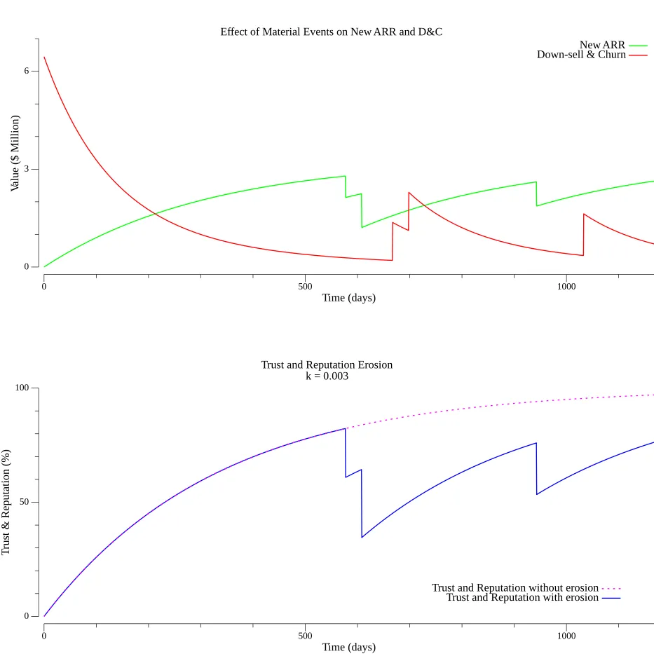
In the example above, where the company experienced three major incidents, the New ARR (green plot) closely follows the trajectory of trust, rising and falling at similar times. This suggests that major incidents can hinder new sales just as they are about to close. On the other hand, D&C behaves oppositely, increasing when trust declines, but with a noticeable delay of around 90 days. This delay likely aligns with a quarterly sales cadence, reflecting how the impact of lost trust filters through contract renewals and customer decisions over time.

ARR and D&C

Monte Carlo Simulations for Predictive Modeling

To understand the potential impact of trust-eroding incidents on D&C and ARR, we use Monte Carlo simulations to generate different event scenarios. This allows us to capture the uncertainty and variability inherent in real-world situations.

Monte Carlo simulations work by generating a large number of possible outcomes based on the probabilistic characteristics of trust-eroding events, such as their frequency and severity. These simulations help us model the evolution of Trust and Reputation over time, which in turn affects D&C and New ARR.

Where to Obtain Data

To build an effective model, you’ll need accurate data on breach frequency and magnitude. Here are some sources to consider:

Research Institutes: Cyentia provides sector-specific data about breaches, leveraging historical data from Advisen. This can give you insights into both the frequency and severity of incidents.
Cyber Risk Quantification Services: Other specialized services may also provide relevant data, often tailored to your industry.
Cyber Insurance Providers: Your cyber insurance company may offer insights into the likely scenarios they consider most damaging for your organization.

Keep in mind that data from these sources will always carry some uncertainty. To address this, you can apply Bayesian updating—a technique that refines your model based on observed data. By grounding your uncertain estimates in actual events, this approach ensures that your future predictions better reflect past financial performance.

A Worked-Out Example

Suppose you have the following estimates regarding your risk exposure:

Average Annual Loss: $900,000
1-in-100 Chance Annual Loss (99th percentile, $P_{99}$ , tail loss): $12,000,000
Annual Event Likelihood: 25%

Loss Magnitude

Since the loss magnitude is expected to be heavy-tailed, we use a log-normal distribution to model it. Here, we’ll derive the parameters of this distribution.

Calculating the Loss Magnitude Distribution Parameters

click to open/close

Consider the loss magnitude as a random variable $M$ , with $\mu$ and $\sigma$ representing the mean and standard deviation of the natural logarithm of $M$ . The average annual loss $E(M) = 900,000$ , which is the arithmetic mean of the log-normal distribution, and the 99th percentile ( $P_{99}$ ) of the loss is $12,000,000$ . These two values relate to $\mu$ and $\sigma$ as follows:

\begin{align} E(M) &= e^{\mu + \frac{\sigma^2}{2}} = 900,000 \nonumber \\ P_{99} &= e^{\mu + z_{0.99}\sigma} = 12,000,000 \nonumber \end{align}

where $z_{0.99} \approx 2.326$ is the 99th percentile of the standard normal distribution.

To solve for $\mu$ and $\sigma$ :

Take the natural logarithm of both equations to linearize them:
$\mu + \frac{\sigma^2}{2} = \ln(900,000)$ $\mu + 2.326\sigma = \ln(12,000,000)$
Solve these two equations:
$\mu + \frac{\sigma^2}{2} = 13.7102$ $\mu + 2.326\sigma = 16.3004$
Rearranging and substituting, we get:

\dfrac{\sigma^2}{2} - 2.326\sigma + 16.3004 -13.7102 =0

This is a quadratic equation of the form $a\sigma^2 +b\sigma +c$ , where $a=\frac{1}{2}, b=-2.326$ and $c=16.3004-13.7102$ . The general solution for $\sigma$ is therefore

\sigma = \dfrac{-b \plusmn \sqrt{b^2 - 4ac}}{2a}= 2.326\plusmn \sqrt{(-2.326)^2 -2(\ln(P_{99}-\ln(E(M))))}

Taking the addition case, we have

\sigma = 2.326 + \sqrt{(-2.326)^2 - 2(16.3004-13.7102)} \approx 2.8053

Substituting in $\mu + 2.326\sigma = \ln(12,000,000)$ gives

\sigma \approx 2.8053, \mu \approx 9.7752

Thus, the parameters for the log-normal distribution are $\mu \approx 9.7752$ and $\sigma \approx 2.8053$ . These values represent the mean and standard deviation of the logarithm of the loss magnitude, which helps in capturing the expected heavy-tailed nature of the risk exposure.

Event Frequency

Given an annual event likelihood of 25%, which indicates a 1 in 4 chance of experiencing at least one event per year, we can model the occurrence of material events in our Monte Carlo simulations using a Poisson process. The expected arrival rate $\lambda \approx 0.288$ is calculated as follows:

Calculating Event Arrival Rate

click to open/close

Deriving the Poisson $\lambda$ parameter

Let $X$ be the random variable representing the number of events per year, and $p$ be the annual event likelihood ( $p=0.25$ in the example). The probability of having at least one event is given by:

P(X \ge 1) = 1 - e^{-\lambda} = p =0.25

Rearranging this equation gives:

e^{-\lambda} = 0.75

Taking the natural logarithm of both sides:

-\lambda = \ln(0.75)

Therefore:

\lambda = -\ln(0.75) \approx 0.2877

This value of $\lambda \approx 0.2877$ represents the expected number of events per year. Thus, over the course of a year, the expected number of loss events is approximately:

\text{Total Expected Events} = \lambda \approx 0.288

This means we expect, on average, 0.288 loss events per year.

Event Time to Live (TTL)

To enhance our trust model, we also incorporate the time it took to recover from an event, referred to as the time-to-live (TTL) of the event. We model this recovery time using an exponential distribution with a rate parameter of $\lambda_{\text{TTL}} = 7$ days. This implies that the expected recovery time is $\frac{1}{\lambda_{\text{TTL}}} = \frac{1}{7}$ days, or approximately 0.14 days.

By incorporating this recovery time, we can simulate the impact of prolonged recovery periods on trust dynamics.

Running the Simulation

With these parameters, we are now equipped to perform our Monte Carlo Simulation.

10,000 Monte Carlo Simulations

click to open/close

Simulation Details

Running a three-year event horizon simulation:

Generate Event Scenarios: The simulation generates thousands of potential future incident timelines, each with different sequences, magnitudes, and frequencies of trust-eroding events.
Model Trust Evolution: For each scenario, we calculate how Trust and Reputation evolve over time in response to incidents. Trust decays after each event and gradually recovers, following our defined trust model.
Estimate D&C and New ARR: Using the trust levels from each scenario, we estimate the average Down-sell and Churn (D&C) and average New ARR over time. Higher trust levels lead to reduced churn and increased ARR, while lower trust levels have the opposite effect. We provide details of how to calculate average D&C and average ARR for a simulation later.

Simulation	Event Day	Magnitude ($)	TTL (Days)	Average ARR ($)	Average D&C ($)
1	205	11.5K	34.36	1.62M	310K
	227	58.2K	0.65
	1095	34.5K	0.50
2	441	1.40K	7.13	2.38M	690K
2	760	434	10.41	2.38M	690K
5	824	13.9K	8.57	1.60M	302K
5	1320	214	5.47	1.60M	302K
6	13	7.24K	27.38	1.59M	294K
	233	92.9K	3.63
	1097	7.53K	23.94
	1131	325K	6.36
7	561	9.47K	7.21	1.90M	448K
7	1277	20.3	5.71	1.90M	448K
…	…	…	…	…	…
9995	62	776	5.90	3.98M	1.49M
9995	359	276	9.91	3.98M	1.49M
9996	739	2.56M	29.77	1.89M	446K
9997	298	3.24K	7.07	1.41M	205K
	939	4.12K	9.82
	1141	17.8K	11.86
	1152	4.87K	6.49
	1439	4.28K	6.47
9998	582	31.4K	4.04	1.60M	300K
	620	143	15.50
	860	481	5.44
9999	337	432K	16.46	1.46M	231K
	366	4.39K	0.74
	526	137K	2.72
	1433	6.66K	5.47

In simulation 1, three loss events occurred within a three-year period, specifically on day 205, day 227 and day 1095. Each event had an associated loss magnitude and a Time to Live (TTL), representing the duration required for recovery. This data is then input into our trust model to assess the impact on New ARR (Annual Recurring Revenue) and D&C (Down-sell and Churn). Using the established model, we calculate the Average ARR and Average D&C over the simulation period, providing insights into the long-term financial effects of these events.

An example of how to calculate the average ARR and D&C for a given Monte Carlo simulation is provided below.

Calculating Average ARR and D&C (warning: integral calculus ahead!)

click to open/close

Steps for calculating ARR and D&C

The analysis below provides the details for calculating average ARR and D&C per simulation. The steps are as follows:

Conduct a Monte Carlo simulation and observe the number $n$ of events that occurred (along with their magnitudes and time-to-live, TTL).
For each $i \in [0, 1, ..., n]$ , calculate the following integrals to compute the total ARR and D&C between consecutive events: $\displaystyle \int_{t_{i-1}}^{t_i} \text{ARR}(t,i) \, dt$ and $\displaystyle \int_{t_{i-1}}^{t_i} \text{DC}(t,i) \, dt$
The averages are:

\begin{align} \displaystyle \frac{1}{n+1} \sum_{i=1}^{n+1} \frac{1}{t_i - t_{i-1}} \int_{t_{i-1}}^{t_i} \text{ARR}(t,i) \, dt \nonumber \\ \displaystyle \frac{1}{n+1} \sum_{i=1}^{n+1} \frac{1}{t_i - t_{i-1}} \int_{t_{i-1}}^{t_i} \text{DC}(t,i) \, dt \nonumber \end{align}

ARR Calculation

The total ARR over the event time interval $[t_{i-1}, t_i]$ is given by:

\begin{align} \int_{t_{i-1}}^{t_i} \text{ARR}(t,i) \, dt &= \int_{t_{i-1}}^{t_i} \left(\text{ARR}_0 \times \alpha(t,i) \times \Tau(t,i)\right) dt \nonumber \\ &= \int_{t_{i-1}}^{t_i} \text{ARR}_0 \times \left(\alpha_0 + \alpha_1e^{-c_\alpha(t-t_i)}\right) \times \left( 1- e^{-k(t - t^i_0)} \right)dt \nonumber \\ &= \text{ARR}_0 \int_{t_{i-1}}^{t_i} \left(\alpha_0 + \alpha_1 e^{c_\alpha t_i} e^{-c_\alpha t}\right) \times \left( 1- e^{k t^i_0} e^{-k t} \right)dt \nonumber \\ &= \text{ARR}_0 \int_{t_{i-1}}^{t_i} \left(\alpha_0 - \alpha_0 e^{k t^i_0} e^{-k t} + \alpha_1 e^{c_\alpha t_i} e^{-c_\alpha t} - \alpha_1 e^{c_\alpha t_i} e^{-c_\alpha t} e^{k t^i_0} e^{-k t}\right) dt \nonumber \\ &= \text{ARR}_0 \int_{t_{i-1}}^{t_i} \left(\alpha_0 - \alpha_0 e^{k t^i_0} e^{-k t} + \alpha_1 e^{c_\alpha t_i} e^{-c_\alpha t} - \alpha_1 e^{c_\alpha t_i + k t^i_0} e^{-(c_\alpha + k) t}\right) dt \nonumber \\ &= \text{ARR}_0 \left[ \alpha_0 t + \frac{\alpha_0 e^{k t^i_0}}{k} e^{-k t} - \frac{\alpha_1 e^{c_\alpha t_i}}{c_\alpha} e^{-c_\alpha t} + \frac{\alpha_1 e^{c_\alpha t_i + k t^i_0} }{c_\alpha + k} e^{-(c_\alpha + k) t} + C \right]_{t_{i-1}}^{t_i} \nonumber \\ &= \text{ARR}_0 \left[ \alpha_0 \left(t_i - t_{i-1} \right) + \frac{\alpha_0 e^{k t^i_0}}{k} \left(e^{-k t_i} - e^{-k t_{i-1}} \right) - \frac{\alpha_1 e^{c_\alpha t_i}}{c_\alpha} \left(e^{-c_\alpha t_i} - e^{-c_\alpha t_{i-1}} \right) + \frac{\alpha_1 e^{c_\alpha t_i + k t^i_0} }{c_\alpha + k} \left( e^{-(c_\alpha + k) t_i} - e^{-(c_\alpha + k) t_{i-1}} \right) \right] \nonumber \\ % &= \text{ARR}_0 \times \left( \alpha_0(t_i - t_{i-1}) - \frac{\alpha_0}{k}\left(e^{-k (t_{i-1} - t^i_0 )} - e^{-k(t_i - t^i_0)}\right) + \frac{\alpha_1}{c_\alpha} \left(e^{-c_\alpha(t_{i-1} - t_i)} - 1\right) - \frac{\alpha_1 e^{c_\alpha t_i + k t^i_0}}{c_\alpha + k} \left( e^{-(c_\alpha + k)t_i} - e^{-(c_\alpha + k) t_{i-1} }\right) \right) \nonumber \end{align}

This expression gives the total ARR for the event time interval, capturing how ARR evolves with respect to trust and recovery dynamics.

D&C Calculation

Similarly, the total D&C over the event time interval $[t_{i-1}, t_i]$ is given by:

\begin{align} \int_{t_{i-1}}^{t_i} \text{DC}(t,i) \, dt &= \int_{t_{i-1}}^{t_i} \left(\text{DC}_0 \times \beta(t,i) \times (1-\Tau(t,i))\right) dt \nonumber \\ &= \int_{t_{i-1}}^{t_i} \text{DC}_0 \times \left( \beta_0 + \beta_1 e^{-c_\beta(t - t_i)} \right) \times \left( 1 - \left(1 - e^{-k(t - t^i_0)} \right) \right ) dt\nonumber \\ &= \int_{t_{i-1}}^{t_i} \text{DC}_0 \times \left( \beta_0 + \beta_1 e^{-c_\beta(t - t_i)} \right) \times e^{-k(t - t^i_0)} dt\nonumber \\ &= \text{DC}_0 \int_{t_{i-1}}^{t_i} \left( \beta_0 e^{-k(t - t^i_0)} + \beta_1 e^{-c_\beta(t - t_i)} e^{-k(t - t^i_0)} \right) dt\nonumber \\ &= \text{DC}_0 \left[ \int_{t_{i-1}}^{t_i} \beta_0 e^{k t^i_0} e^{-k t } dt + \int_{t_{i-1}}^{t_i} \beta_1 e^{c_\beta t_i +k t^i_0} e^{-(c_\beta + k)t} dt \right] \nonumber \\ &= \text{DC}_0 \left[ -\frac{\beta_0 e^{k t^i_0}}{k} e^{-k t } - \frac{\beta_1 e^{c_\beta t_i +k t^i_0} }{c_\beta + k} e^{-(c_\beta + k)t} + C_0 \right]_{t_{i-1}}^{t_i} \nonumber \\ &= -\text{DC}_0 \left[ \frac{\beta_0 e^{k t^i_0}}{k} e^{-k t } + \frac{\beta_1 e^{c_\beta t_i +k t^i_0} }{c_\beta + k} e^{-(c_\beta + k)t} + C_0 \right]_{t_{i-1}}^{t_i} \nonumber \\ &= -\text{DC}_0 \left[ \frac{\beta_0 e^{k t^i_0}}{k} \left( e^{-k t_i } - e^{-k t_{i-1} } \right) + \frac{\beta_1 e^{c_\beta t_i +k t^i_0} }{c_\beta + k} \left( e^{-(c_\beta + k)t_i} - e^{-(c_\beta + k)t_{i-1}} \right) \right]\nonumber \\ &= \text{DC}_0 \left[ \frac{\beta_0 e^{k t^i_0}}{k} \left( e^{-k t_{i-1} } - e^{-k t_i } \right) + \frac{\beta_1 e^{c_\beta t_i +k t^i_0} }{c_\beta + k} \left( e^{-(c_\beta + k)t_{i-1}} - e^{-(c_\beta + k)t_i} \right) \right]\nonumber \\ \end{align}

This expression captures the total D&C between two events, reflecting how customer down-sell and churn evolves with respect to the damage to trust and the defined recovery dynamics.

Conclusion

The results of the Monte Carlo simulation offer a powerful tool for predicting the probability of various financial outcomes, enabling decision-makers to assess the potential impact of cybersecurity events on business objectives. By analyzing the range of possible outcomes, organizations can gain a clearer understanding of potential financial risks and better prepare for uncertainties, enhancing their ability to make informed decisions and develop more effective mitigation strategies.

Happy Modeling and Decision-Making!

Trust on the Line:

Modeling the Financial Impact of Cybersecurity Failures.

Why Model the Fallout of Reputation Risks on Financial Outlook?

The Economics of Trust and Reputation

Supporting Decision-Making

Modeling Trust and Reputation

Modeling the Trust Impact of a Loss Event