· Dayo Adetoye (PhD, C|CISO) · Partnering with the Business · 31 min read
Security Investment as Board Strategy:
Pricing Protection on Both Sides of the Boom.
Beyond the Boom gave every security control two scores: TMP for preventing loss events, LMAP for limiting the damage when they happen. This sequel prices them, scenario by scenario: two closed-form Bayesian updates - one for how often loss events happen, one for what they cost - feeding a per-control return calculation, credited across every scenario a control covers, that a board risk committee can follow line by line. The board conversation shifts from whether security spend is justified to which priced option gets funded first - with the board owning the loss threshold, the price of tail risk, and the review cadence. An interactive calculator runs the method on your own numbers.
In my last post I argued that a mature security program dual-scores every control: how well it keeps the boom from happening (Threat Mitigation Potential), and how well it limits the damage when the boom arrives (Loss Magnitude Attenuation Potential). The board narrative that came with it - brakes and airbags - has worked every time I’ve used it.
Brakes and airbags name the two kinds of protection. Pricing them is the open question: should the next dollar go to immutable backups or to phishing-resistant multi-factor authentication (MFA)? Is the incident-response retainer worth more than extra endpoint detection and response (EDR) coverage? The framework as published classifies controls. It can’t yet rank purchases. This post adds that.
The approach: one closed-form Bayesian update for how often events happen, one for what they cost, and a per-control return calculation a board risk committee can follow line by line. The method is deliberately simple - tractable and defendable beats precise. Your inputs are expert estimates and a handful of real incidents; elaborate math on top of them adds fragility, not accuracy. Every step here can be checked by hand and defended in one sentence.
In This Post
The collapsed guides along the way hold the reproduce-it-yourself detail.
- Where We Left Off: Brakes, Airbags, and One Equation
- The Engine: Start With the Industry Number, Let Your Own History Pull It
- One Number to Update, Six Ways to Spend It
- Qualify Before You Quantify
- A Worked Example: Three Scenarios, Four Controls
- One Control, Several Scenarios
- The Boom ROI Calculator
- From a Ranking to a Strategy
- What the Board Owns
- Board Talking Points for CISOs · CISO Takeaways · Closing
Where We Left Off: Brakes, Airbags, and One Equation
The boom is the moment a loss event materializes - ransomware detonates, the data leaves. Everything left of boom reduces how often events happen - loss event frequency (LEF); everything right of boom reduces how much they cost - loss magnitude (LM). Pure shields (MFA, patching) work only on frequency. Pure shock absorbers (backups, insurance, crisis communications) work only on magnitude. Hybrids (segmentation, EDR) work on both. One equation ties it together:
In words: expected loss is event frequency times the expected cost per event, with each control cutting its share from one side or the other. The sections below put dollars and evidence behind each term.
The Engine: Start With the Industry Number, Let Your Own History Pull It
No single firm has enough incidents to estimate its own loss rates from scratch. What you have is industry data plus a short internal history, and Bayesian updating is built for exactly that combination. The unit of analysis is the scenario - a named loss-event class such as ransomware, data breach, or business email compromise (BEC). Each scenario gets its own frequency update, its own magnitude update, and its own loss overlay; the judgment parameters are set once and shared across all of them. Public sources publish organization-level views rather than per-scenario rates; the second practitioner’s guide below turns one into the other.
Frequency (left of boom). Start with an industry base rate for the scenario - public sources such as the Cyentia IRIS studies give you a credible starting frequency, call it λ (lambda), the expected number of events per year. Then let your own record pull that number:
Two of these inputs are facts about your data: the event count is how many events of this class your firm actually had, and the years of history is your observation window - fractional, because each quarterly re-run extends it by a quarter-year, and new events join the count as they occur. The window’s bounds are real: shorter throws away scarce evidence, and longer updates today’s estimate with data from a company that no longer resembles you (different stack, different threats, different controls).
That leaves one judgment call: β₀ (beta-zero), how many years of your own experience the industry benchmark is worth - a question a board member can reason about directly. β₀ = 30 against a six-year window says the industry dataset counts for five times your own history: informative because it covers thousands of firms, capped because it averages over what makes your firm different. Publishing the sensitivity range keeps the judgment visible - run the update at β₀ = 10 and at 100 and show the band the answer moves in. On those settings, one bad year moves the estimate without owning it, and the whole update stays one line of arithmetic a numerate member of the board’s risk committee can check on a phone calculator.
Magnitude (right of boom). The mirror image, run on what events cost. Anchor each scenario with industry percentiles - a median cost (P50, the middle outcome) and a plausibly-bad cost (P95, the one-in-twenty outcome) - and let your own fully-costed incidents pull the anchor. Because losses are lopsided (many moderate, a few enormous), the blend happens on the logarithm of cost, but the shape is identical:
The parameter is m₀ (m-zero), the same judgment on the loss-size side: how many observations of loss size is the industry anchor worth? m₀ = 5 says the anchor counts for five of your own fully-costed events - a deliberate discount, because the anchor aggregates many incidents but they are other firms’ losses, most missing cost data entirely and the rest skewed toward direct, publicly visible costs, while one costed event of your own captures your actual cost structure. Trusting the anchor as five of yours rather than fifty prices that gap: one costed incident shifts the anchor by a visible margin without dominating it, and m₀ gets the same published sensitivity range as β₀.
Two mechanics close the magnitude side, stated here in brief and specified fully in the foldable below. First, per-event cost is modeled as lognormal - the standard shape for losses where many are moderate and a few are enormous - and a scenario’s expected annual loss uses the lognormal mean, which sits above the median because the rare enormous losses pull the average up. That gap is material: in the worked example below, the ransomware anchor updates to $2.89M while the expected cost per event is $4.12M. Second, every estimate in the method ships with a 90% credible interval, computed from the same closed-form posteriors by sampling them - 90% being the decision-analysis convention that matches the P50/P95 anchor pair. With one or two observations the intervals are wide - that is the honest state of the evidence - and each quarterly re-run narrows them as history accumulates.
β₀ and m₀ are judgments you can make defensibly in thirty minutes. Five rules of thumb and one grounding fact about the source, stated for β₀ and then carried over to m₀ at the end:
0. Know your source’s population. IRIS 2025 describes its methodology as counting incidents that reached the public record - breach disclosures, regulatory filings, litigation, freedom-of-information requests - so significant events are well represented and minor ones are not. Two practical consequences. First, count k - your event count - against that population: it must be material events of the kind that would surface publicly, because counting every internal near-miss against a disclosed-events prior mixes populations and inflates the posterior. Second, the prior leans high by design - IRIS reports the risk-averse upper-bound estimate, with organizations in its incident database as the denominator rather than all firms that exist - so a clean internal history pulling your posterior below the benchmark is the update working correctly with a conservative prior, worth saying when someone challenges the direction of movement.
1. Start at 30, adjust once. Set the prior mean before pricing it: IRIS 2025 publishes incident likelihood by sector and by revenue band as separate views - annual probability curves for each, plus each cohort’s multiplier relative to the overall median - so build your slice by applying the sector and size multipliers to the base rate, the same construction this article’s priors use. β₀ then prices how typical your firm is within that slice, and the estimates themselves come from random-effects models, which pull thin cohorts toward the overall average - a finely sliced number rests on fewer observations than it appears to. Ask one question: how typical is my firm of the cohort behind the number?
| Within-slice typicality | β₀ range | Rationale |
|---|---|---|
| Typical - a representative member of a well-populated slice: digital footprint, threat profile, and control maturity near cohort norms | 30–50 | The slice average genuinely describes firms like yours |
| Atypical or thin - right slice, but your footprint or threat profile diverges from cohort-typical, or the slice is thin enough to lean on model smoothing | 15–30 | The number is informative; the cohort average isn’t you |
| Straddling - no published slice genuinely contains you: post-M&A hybrid, niche sub-industry inside a broad sector bucket | 8–15 | Let your own data speak faster |
2. Let your rarest scenario anchor the choice. β₀ is shared across all scenarios: one value for the whole model. A β₀ that works for a common scenario (BEC, where you have several internal events) may be too weak for a rare one (nation-state, regulatory breach) where zero events and a low β₀ would price the threat near zero. Anchor β₀ to the rarest scenario in your portfolio: if 30 keeps the rare-scenario posterior at a rate you still believe, it will behave well on the common scenarios too, because those have enough internal events to pull the estimate regardless. One exception class is allowed: a scenario may take its own, usually lower, prior strength when it fails a stated test - the source does not genuinely publish that event class, or the anchor is expert-estimated rather than data-backed. Record each exception with a one-sentence rationale, the same discipline as the measure/exclude gate; expect one or two in a typical portfolio, not one per scenario. The sensitivity sweep runs on the shared value, exceptions stay pinned and noted, and the board framing holds: two shared prior strengths, with one documented exception where the industry data is thin.
3. The “three bad years” gut check. After picking β₀, imagine three consecutive events in three years. Does the posterior land somewhere you’d actually believe? Starting from the worked example’s ransomware row - λ prior = 0.04, one event already in the six-year window - three more events in three years makes the event count k = 4 over an observation window T = 9 years, which gives:
- β₀ = 10 → λ posterior ≈ 0.23 (one in four years - your bad streak dominates)
- β₀ = 30 → λ posterior ≈ 0.13 (one in eight years)
- β₀ = 60 → λ posterior ≈ 0.09 (one in eleven years - the prior barely moves)
If the gut-check rate feels right for a firm that just had three events, your β₀ is calibrated.
4. The sweep is the deliverable. Run the model at β₀ = 10, 30, and 100. If the ROSI ranking is stable across the sweep, the exact value doesn’t matter for the decision - report the band. If the ranking flips, that is the finding: the purchase depends on a judgment you haven’t resolved, and you need more data or a tighter cohort match.
5. Document in one sentence; revisit on structural change. Record your β₀ with its rationale and the IRIS edition used. Example: “β₀ = 30, IRIS 2025 mid-market information-services cohort. We match on industry and revenue band; control maturity above-median. Sensitivity sweep at 10/30/100 shows the top-two ranking stable.” Revisit when something structural changes - M&A, platform migration, a new regulatory regime - and at most annually. The natural decay is built in: as T grows each quarter, β₀’s share of the denominator shrinks automatically.
The same five rules apply to m₀, with costed events in place of years of history. The framing question becomes: how many of my own fully-costed events is the industry anchor worth? Start at 5 and adjust once, on anchor provenance:
| Anchor provenance | m₀ range | Rationale |
|---|---|---|
| Data-backed pattern-level percentiles, scaled to your revenue tier | 5–10 | The anchor rests on real loss data shaped to firms your size |
| Pattern-level but unscaled, or a partial match to your scenario | 3–5 | Real loss data whose shape doesn’t fit your firm - discount accordingly |
| Expert-estimated anchor (no published loss data for the class) | 1–3 | Your first real costed event should dominate - record as a rule-2 exception |
The one-event gut check. Suppose your first fully-costed event comes in at three times the anchor’s median. Because the blend runs in log-cost, the posterior median rises by a factor of 3 raised to the power 1/(m₀ + 1) - the event’s threefold excess, shared across the anchor’s weight plus your one observation:
- m₀ = 1 → the median rises 73% (the single event owns the anchor)
- m₀ = 3 → +32%
- m₀ = 5 → +20%
- m₀ = 10 → about +10% (the anchor barely concedes)
Pick the movement you would defend to the board after one bad event. At m₀ = 5, your own data carries one-sixth of the weight after one costed event, two-sevenths after two, and half at five.
m₀ has no automatic decay. The exception test from rule 2 matters more here than on the frequency side: data-rich scenarios rescue a misfit β₀ through their event count, but costed-loss observations number zero to two everywhere, so m₀ always dominates the magnitude blend. β₀’s influence also decays on its own - T grows every quarter whether or not events occur - while m₀ cedes weight only when you actually cost an event, which may be years apart. A misjudged β₀ corrects slowly by itself; a misjudged m₀ waits for data that may not come. When uncertain, set m₀ low rather than high: an anchor that concedes too much weight is corrected by your next costed event, while an anchor that concedes too little holds its error until enough of your own costed events accumulate to outweigh it. If any prior-strength exception earns its place it is a magnitude-side one - an expert-estimated anchor should yield to the first real costed event, and a low m₀ does exactly that.
Sweep and document, as in rules 4 and 5. Run the magnitude update at m₀ = 3, 5, and 10 - the sweep is the deliverable here too - and record the choice in one sentence naming the anchor’s provenance. Example: “m₀ = 5, IRIS 2025 pattern-level percentiles scaled to our revenue tier - data-backed and size-adjusted. Sweep at 3/5/10 leaves the ROSI ranking stable.” One caveat inherited from the source: IRIS loss data skews toward direct, publicly visible losses - response costs, lost revenue, class actions - and rarely captures indirect or intangible impacts, which is why reputation and competitive-advantage dollars live in your overlay as your own estimates rather than in the industry anchor.
The severity model. The anchor pair pins the lognormal down: σ (sigma), the spread of log-cost, is (ln P95 − ln P50) ÷ 1.6449, where ln is the natural logarithm and 1.6449 is how many standard deviations separate a normal distribution’s median from its 95th percentile. σ is held fixed through the update, because one or two observations cannot support learning a spread, so the P95 moves in proportion to the median. A scenario’s expected annual loss is then λ × the lognormal mean, e^(µ + σ²/2) with µ (mu) the log of the updated median. Skipping the mean and multiplying λ by the median anchor understates expected loss by exactly the skew factor e^(σ²/2) - on the worked example’s ransomware row, $176.6K instead of $252.0K.
The credible intervals. Both posteriors have named closed forms: the event rate’s posterior is a Gamma distribution with shape β₀ × λ_industry + your event count and rate β₀ + your years of history, and the log-cost center’s posterior is a Normal distribution around the updated log-median with variance σ² ÷ (m₀ + your number of costed events). The procedure: draw a few thousand seeded (λ, µ) pairs per scenario, compute the expected loss each pair implies, apply the control factors, and read the 5th and 95th percentiles off the results.
IRIS 2025’s likelihood views are organization-level: they estimate the chance that a firm like yours has an incident, not a ransomware incident specifically. Its event-type data is population-level: the mix of incident patterns and their loss distributions across all firms. Per-scenario priors come from combining the two. Six steps:
1. Start with your slice’s total rate. The sector and size views give p, the annual probability that a firm like yours has at least one incident. Convert it to a total event rate, λ_total = −ln(1 − p) - ln is the natural logarithm, and λ_total is the event rate that makes “at least one event” come out at exactly p; at these probabilities it is barely larger than p itself. λ_total is the budget your scenarios share.
2. Apportion by the event-type mix. IRIS 2025 publishes the relative frequency of its incident patterns across the whole population, tracked over time; it does not condition the mix on sector or size. Split the budget: λ_scenario = λ_total × that scenario’s share of incidents, using the most recent mix rather than a long-run average - the mix moves (ransomware went from a sliver to more than a third of incidents within a decade). Population-wide shares are acceptable when your sector’s threat mix is near-typical; where it demonstrably skews (payment-card fraud in retail, denial-of-service against utilities), adjust the affected shares and record the reasoning.
3. Map the taxonomy explicitly. Your scenario list will not match IRIS’s nine patterns one-to-one (accidental disclosure, DoS attack, defacement, fraud or scam, insider misuse, physical threats, ransomware, system failure, system intrusion). Write the mapping down: this article’s data breach takes system intrusion plus accidental disclosure; its BEC takes fraud or scam. Shares must sum to 1 across your list, and a scenario that aggregates two patterns takes the sum of their shares. A documented mapping is auditable; an implicit one is where models quietly break.
4. Scenarios the source doesn’t cover. Emerging classes - AI security is the canonical example - have no published share. Assign a share by expert estimate, take it out of the residual so the total still sums to 1, and treat the scenario as a prior-strength exception under the first guide’s rule 2: the source does not genuinely publish that event class.
5. Magnitude anchors per scenario. IRIS 2025 publishes loss distributions per incident pattern - median and 95th-percentile markers, plus per-pattern trend lines - at the whole-population level, not conditioned on size. Take the pattern-level percentiles as starting anchors and scale them by the size-loss relationship the report does publish (loss statistics by revenue tier): the ratio of your tier’s median to the all-firm median is the adjustment. Sanity-check the result: the frequency-weighted blend of your per-scenario anchors should sit near the slice-level loss picture, and a mismatch means your mix or your anchors are off.
6. Document the whole chain in one place - slice chosen, λ_total, shares and their source figure, taxonomy mapping, expert-estimated residuals, anchor sources - so the quarterly re-run repeats it mechanically. Example: “Information sector × $10M–$100M tier; λ_total from the sector and size views; shares from the latest pattern mix; data breach = system intrusion + accidental disclosure; AI security 5% by expert estimate from the residual, m₀ exception recorded; anchors from pattern-level percentiles scaled to our revenue tier.”
With one or two internal data points, a moderately strong prior is correct: one observation should update the estimate without dominating it. β₀ and m₀ are the only judgment parameters in the estimation engine - every other input is your own data or public industry data - and a third and final one, a stated price on tail-risk reduction, arrives with the control ranking later in the post. Re-run the update quarterly; each quarter’s posterior becomes the next quarter’s prior.
Positioning the Model to the Board
Board Message: “This model asks the board for three decisions, and only three: the loss threshold that matters - already set through our insurance retention and materiality - the price we put on reducing tail risk, and the cadence on which we re-run and review. We optimize within those and bring back the trend.”
What this gives the board:
- The board sets the objective function; the security team runs the optimization
- The loss threshold is inherited from decisions the board has already made
- Risk appetite becomes a published number the ranking visibly responds to
- Oversight is a quarterly trend read: intervals narrowing, ranking stable
One Number to Update, Six Ways to Spend It
The magnitude update runs at the aggregate dollar level - one update per scenario, on the total cost of an event. Decisions need more detail than a total, so each scenario’s cost also carries a decision overlay: the six forms of loss from Factor Analysis of Information Risk (FAIR) - response cost, replacement cost, productivity loss, fines and judgments, reputation damage, and competitive advantage loss - each with its estimated share of the dollars.
Form-level data is far scarcer than event-level data: you will almost never have enough observations per form to update six cells credibly, and no decision requires it. The overlay serves two specific decisions:
- Control targeting. Each post-boom control attenuates specific forms of loss. Immutable backups compress downtime and response dollars and never touch fines. Crisis communications works on reputation only. The overlay turns that specificity into the dollar terms the ranking uses.
- The insurance read. The overlay shows which of a scenario’s dollars your policy can reach, which sit below the retention, and which no policy covers.
The Insurance Read
Board Message: “Of the expected cost of this scenario, here is the share our insurance can actually reach - and here is the share no policy structure will cover, because reputation and competitive-position losses are largely uninsurable. That uninsurable share is what our resilience investments defend.”
What the overlay makes readable:
- Insurable vs. uninsurable dollars, per scenario
- Which forms sit below the retention (self-insured in practice)
- Where sublimits bind before the headline limit does
- Which findings belong in renewal negotiations
Qualify Before You Quantify
Not every form of loss is relevant, measurable, or worth measuring for every scenario. Filling every cell anyway loads the model with numbers no evidence supports. Before any number enters the overlay, run a four-step gate:
- Which forms apply here - and which demonstrably don’t?
- For each form that applies, what would concretely happen? Describe the loss mechanism in specific terms.
- Measure it, or consciously exclude it - three-leg test: is it material, is it obtainable, does it change a decision? If a leg fails, record which one.
- Name the data source for everything you commit to measure: finance general-ledger coding, legal matter billing, incident-response retainer invoices, insurance-broker claims data, IT operations downtime metrics.
The test case is reputation damage: it applies to almost every scenario and is measurable in almost none. Customer attrition takes quarters to appear and is confounded by everything else the company did that year. Record the exclusion, note the failing leg (obtainability), name the trigger that would reopen it, and move on. The record of why you excluded a form is itself useful output: an auditor can inspect the reasoning, and the model stays free of numbers nobody can defend.
Collect incident costs form-by-form regardless - the invoices are already itemized. The form-level dollars sum to the single aggregate observation the Bayesian update needs, and the same collection refreshes the overlay split.
A Worked Example: Three Scenarios, Four Controls
The example firm is a fictional mid-market information-services company; every number is invented for illustration. Three scenarios - ransomware, data breach, business email compromise - share one judgment set: β₀ = 30, a six-year window, m₀ = 5.
Ransomware. Industry prior of one disruptive event per twenty-five firm-years (λ = 0.040). The firm had one event in its six-year window, so the updated frequency is (30 × 0.040 + 1) ÷ 36 ≈ 0.061 events per year. Magnitude anchors: $3.0M median, $12M at the one-in-twenty mark; the event was fully costed at $2.4M, and with m₀ = 5 the anchor settles at $2.89M - an expected cost per event of $4.12M once the lognormal spread is applied. The overlay on the $3.0M anchor is dominated by productivity and response dollars, with reputation and competitive advantage carried as documented exclusions, failing the obtainability leg. Expected annual loss before new controls: 0.0611 × $4.12M ≈ $252.0K.
Data breach is the data-poor case: prior λ = 0.060 and zero events in the window - six clean years are themselves evidence, so the frequency edges down to 0.050, while the magnitude anchor stands at its $1.5M prior with no costed events to move it. Expected annual loss $107.0K; the overlay, the gate, and the control pricing run unchanged on the prior.
Business email compromise: prior λ = 0.100 with two events in six years lifts the frequency to 0.139; one event costed at $250K pulls the anchor from $400K to $370K. Expected annual loss $64.2K. Aggregate across the three scenarios: $423.1K a year (90% credible interval $166K–$888K).
Each overlay sums to its P50 anchor, with excluded forms noted; the calculator ships these values as its defaults.
| Scenario | λ prior; event count | P50 / P95 | Costed events | Overlay dollars |
|---|---|---|---|---|
| Ransomware | 0.040; 1 | $3.0M / $12M | $2.4M | $1.05M productivity, $900K response, $450K replacement, $300K fines (excluded: $200K reputation, $100K competitive advantage) |
| Data breach | 0.060; 0 | $1.5M / $6.0M | none | $500K response, $500K fines, $100K productivity (excluded: $300K reputation, $100K competitive advantage) |
| Business email compromise | 0.100; 2 | $400K / $1.2M | $250K | $280K replacement, $60K response, $40K productivity (excluded: $20K reputation) |
Four candidate purchases. Phishing-resistant MFA: a pure shield, cutting event frequency 35% in all three scenarios, $120K a year. Immutable backups with tested restores: a pure shock absorber, ransomware only, attenuating 50% of the dollars in the forms it touches - productivity, response, replacement: $2.4M of the $3.0M overlay, and none of the fines - for an effective attenuation of 0.40, at $90K a year. That instance follows the general rule: a control’s effective attenuation in a scenario is its LMAP × (measured overlay dollars in the forms it touches ÷ the scenario’s total overlay dollars), where excluded forms drop out of the numerator but stay in the denominator. An incident-response retainer: a shock absorber covering all three scenarios, attenuating 20% of the dollars in response and productivity, $60K. Data loss prevention (DLP) tooling: a hybrid, data breach only, cutting event frequency 15% and attenuating 25% of the dollars in fines and response, $80K. Against data breach’s fines-heavy overlay, the same backups would attenuate a smaller share of the dollars - backups never touch fines - so one control carries a different price in each scenario it covers.
Run the full portfolio and aggregate expected annual loss falls from $423.1K to $170.5K (90% interval $74K–$342K) - $252.7K a year removed. Price each control by asking what expected loss it removes given everything else stays bought, per dollar of annual cost - a return on security investment (ROSI) figure.
One Control, Several Scenarios
Controls differ in coverage. Backups protect ransomware and nothing else. MFA suppresses the credential-and-phishing entry path in all three scenarios. Score both inside the ransomware row and backups win comfortably: $57.0K of expected loss removed per year against $90K of cost (0.63 per dollar), versus MFA’s $46.0K against $120K (0.38). Score them against the aggregate and the order reverses: MFA earns $46.0K in ransomware, $24.4K in data breach, and $21.3K in business email compromise - $91.8K in total (the parts carry rounding), 0.76 per dollar, first in the ranking. The full table, marginal reduction and then return: MFA $91.8K and 0.76, backups $57.0K and 0.63, the incident-response retainer $18.8K and 0.31, DLP $18.7K and 0.23. Each figure carries its credible interval, and the top two overlap - MFA 0.76 (0.33–1.54), backups 0.63 (0.11–1.69) - so the ranking is a best estimate under stated uncertainty. The overlap is itself decision information: collect more cost data, or fund both.
Both scores are correct; they answer different questions. The practical rule: rank controls on aggregate expected-loss reduction per dollar, and read the per-scenario breakdown to see where the credit comes from. A control scored inside a single scenario is understated by exactly the scenarios the scoring left out.
One stated simplification: the aggregate treats scenarios as independent. Real scenarios share kill chains - the phished credential that starts a ransomware event also starts a data breach - and correlation raises the value of upstream, shared controls further. On this model, the independence figure is a floor for a control like MFA; correlation is portfolio context.
Want to run the method on your own numbers? Try the interactive Boom ROI Calculator below.
The Boom ROI Calculator
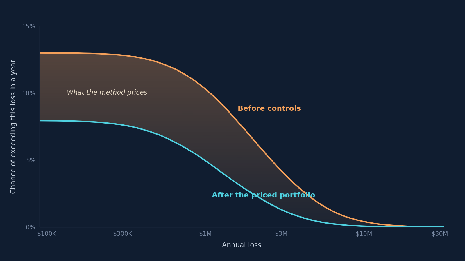
The calculator runs the full method: three default scenarios (ransomware, data breach, business email compromise) and four controls - add or remove your own. Each scenario carries both Bayesian updates and its six-forms overlay with measure/exclude toggles; each control maps to the scenarios it covers; the ROSI ranking runs against the aggregate with a per-scenario breakdown, a left/right-of-boom split bar on every control, and an input for the tail-relief weight defined in the next section; and the annual-loss exceedance curves come from a 10,000-trial Monte Carlo over the whole portfolio - each trial year draws a Poisson event count and lognormal per-event losses per scenario and sums them - with the axis truncated where the pre-control curve drops below one-in-a-thousand, disclosed on the chart. Every headline result carries its 90% credible interval - switchable to 95% if that is your house convention - the attribution view reconciles marginal contributions plus shared reduction to the total removed, and every scenario and control row carries an on/off toggle for what-if analysis, with an impact line comparing the full configuration to the current selection. The defaults reproduce every number in the worked example, so you can check the article’s arithmetic before entering your own data.
From a Ranking to a Strategy
A ranking built on expected loss alone prices the average year, and it undervalues controls whose main contribution is capping the catastrophic year - the P95 annual loss, the one-in-twenty outcome that drives insurance towers and board attention. If that protection has value to your organization, the method prices it explicitly: w, the tail-relief weight, is that price - the dollars of value you assign per dollar of P95 reduction. w is the third and final published judgment parameter, alongside β₀ and m₀; its default is zero, the example above runs at w = 0, and setting it is a board decision - the What the Board Owns section below picks up why.
The formula behind the ranking: toggle a control out of the portfolio across every scenario it covers, observe what comes back, and divide by annualized cost:
Δ (delta) marks a toggle-out difference. ΔEL is the expected annual loss that returns if the control is removed while everything else stays bought - the marginal reduction reported throughout the example. ΔP95 is the same toggle-out read on the 95th-percentile annual loss: remove the control, re-read the P95, take the difference. The stated tail-relief credit is w × ΔP95, and at w = 0 the formula reduces to the pure expected-loss return the example’s figures use. At w = 0.05 - five cents per dollar of P95 reduction - the example’s returns move: MFA reaches 1.00 and backups rise from 0.63 to 0.73, on P95 reductions of about $564K and $166K respectively. The order holds here because the shared shield also prevents the years in which losses stack; in a portfolio whose tail protection is concentrated in one shock absorber, a positive w is what makes that control climb the ranking.
Control effects compound - two 40% controls don’t give you 80% - so standalone valuations double-count shared headroom. Price each control marginally: toggle it out with everything else bought.
Marginal figures deliberately do not sum to the total: across the example portfolio, the four controls’ marginal contributions add to $186.2K while the portfolio removes $252.7K. The $66.5K difference is reduction that overlapping controls would each deliver on their own, so it is credited to none of them. The calculator shows the reconciliation line: marginal contributions plus shared reduction equals total removed.
The marginal reduction also answers where the protection sits: each control’s dollars split into left of boom (fewer events, from its TMP) and right of boom (smaller events, from its effective attenuation), with the interaction between the two sides divided evenly by averaging the two orders in which they could apply. Across the example portfolio, the $252.7K removed is $100.6K left of boom, $85.7K right of boom, and $66.5K shared between overlapping controls. Per control: MFA’s dollars sit entirely left of boom, backups’ and the retainer’s entirely right, DLP’s split 47/53. Per scenario the split is a flag: business email compromise’s reduction is 91% left of boom - nearly all prevention - the visible signal that its damage-limitation side is thin.
The portfolio question follows: per threat, do I have adequate strength on both sides of the boom - and am I buying the next unit of strength at the best marginal rate? A threat with strong prevention and no damage limitation stays exposed no matter how many additional shields you buy. The ROSI ranking prices the next unit of protection; the per-scenario boom split tells you where it is needed.
What the Board Owns
The method draws a division of labor: the board owns the objective function, and the CISO owns the optimization. Exactly three decisions in the model are board-level.
The loss threshold that matters. The board already sets it, through the insurance program’s retention and the company’s financial materiality line; the model inherits that threshold rather than inventing a new one. Every scenario and control is priced against a bar the board has already voted on.
The price of tail risk. Boards state risk appetite in adjectives - “conservative on catastrophic outcomes” - and w, the tail-relief weight from the ranking formula, turns the adjective into a number. A board that says it is conservative about catastrophic outcomes is saying w is greater than zero, and the method asks it to say how much; the ranking re-sorts in view of the answer, visibly.
The cadence and the trend. Re-runs land quarterly, on the financial-reporting rhythm. Board oversight is reading two trend lines - are the credible intervals narrowing, is the ranking stable - rather than reacting to each week’s incident headlines.
The arrangement has a name boards already know: an investment policy statement. The board sets the objectives and constraints, the manager optimizes within them, and performance is reviewed on a cadence against the stated objectives. Run security investment the same way and “security investment as board strategy” is literal: the board sets the threshold, the tail price, and the cadence; the ranking that comes back is the optimization executing that mandate.
Board Talking Points for CISOs
Board Talking Points
“The loss threshold in this model is one the board has already set: our insurance retention and our materiality line. Every scenario and control is priced against it.”
“The price of tail risk is yours to set, as a number. Today it runs at zero; a board that is conservative about catastrophic outcomes is naming a price above zero, and the ranking re-sorts to show what that conviction buys.”
“Oversight runs on the reporting calendar: quarterly re-runs, with two trend reads - the intervals should narrow as our history accumulates, and a stable ranking means the judgment calls are not driving the purchase order.”
“The question in front of this committee changes: from whether security spend is justified to which of these priced options we fund first.”
CISO Takeaways
- Dual-score every control (TMP and LMAP) - then price the marginal dollar
- Two closed-form updates and three published judgment parameters (β₀, m₀, and the tail price w): the updates auditable in one line each
- The scenario is the unit of analysis: per-scenario updates at the whole-event dollar level, a six-forms decision overlay per scenario, judgment parameters set once and shared
- Every estimate ships with a 90% credible interval; overlapping intervals are decision information
- Qualify before you quantify: record exclusions with the failing leg and a revisit trigger
- Rank controls on aggregate expected-loss reduction per dollar; read the per-scenario breakdown for where the credit comes from, and the boom split for which side of the boom the dollars sit on
- The board owns three decisions - the loss threshold it has already set, the tail price w, and the review cadence; everything else is delegable estimation
- Re-run quarterly: each posterior becomes the next prior
Closing: Priced, Published, Re-run Quarterly
Part one named the two kinds of protection. Now both carry prices: cost per unit of protection on each side of the boom, per control, with the three judgment parameters published and the numbers re-run each quarter as your own history accumulates.
The division of labor is what makes this board strategy: the board sets the loss threshold it already owns, the price it puts on tail risk, and the cadence of review; the CISO returns a ranking that executes that mandate.
That shifts the board conversation from whether security spend is justified to which of the priced options gets funded first.