Foundational Metrics and Key Risk Indicators:

Situational Awareness

If you know the enemy and know yourself, you need not fear the result of a hundred battles. If you know yourself but not the enemy, for every victory gained you will also suffer a defeat. If you know neither the enemy nor yourself, you will succumb in every battle.

— Sun Tzu, The Art of War

The first step in understanding your organization’s risk exposure is to have a clear view of your drivers of risk: vulnerabilities. Whether caused by design and architectural flaws, bugs, or misconfigurations, vulnerabilities create opportunities for adversaries to exploit your system and cause damage.

The enemy within

Vulnerabilities are the enemies within, creating the window of opportunity for adversaries inside and outside.

While the presence of vulnerabilities does not guarantee that risks will materialize, but their presence is a precursor and leading indicator to a more likely future materialization of risk.

Our goal is to identify these vulnerabilities and turn them into metrics and Key Risk Indicators (KRIs) that can give us predictive insights for understanding our current risk posture and for decision-making on how to reduce the likelihood of risk materialization through the successful exploit of the vulnerabilities. The metrics are also lagging indicators of our vulnerability management processes that could suggest poor performance or lack of capacity to keep the vulnerability arrival, durability, and growth rates at bay.

This article provides a modelling technique that helps us to reason about leading risk indicator and capacity and performance issues of our vulnerability and risk management program.

A Vulnerability Risk Indicator (VRISC)

Vulnerabilities drive the susceptibility of our system to attacks, which in turn materializes risk. We define a key risk indicator, which we call Vulnerability Risk Indicator Score, or VRISC, that describes our environment’s or asset’s or system’s susceptibility to exploits as follows:

\text{VRISC}_t = 100 \times \left(1 - e^{-5 \tau(\bf V_t,\kappa_{\tiny V}) \times \tau(\text{\bf TTL}_t,\kappa_{\tiny T}) \times \tau(\text{\bf EPSS}_t,\kappa_{\tiny P})}\right)

where $\tau$ is a risk tolerance function defined as

\tau(X, \kappa) = \dfrac{X}{X+\kappa}

The tolerance parameter $\kappa$ in the risk tolerance function $\tau(X, \kappa)$ represents the value of $X$ at which half of the maximum impact on the VRISC score is realized. Essentially, $\kappa$ controls the sensitivity of the VRISC score to changes in $X$ , determining how quickly the score increases as $X$ grows.

Understanding risk tolerance

click to open/close

Risk Aversion and Tolerance factor

The risk tolerance function $\tau$ helps align acceptable risk levels with the business’ risk appetite.

The table below offers a structured way to assess risk appetite for any metric, such as EPSS, Time to Live (TTL), or vulnerability count. For illustration, we use the number of vulnerabilities.

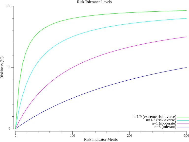
In this example, $X$ represents the number of vulnerabilities, and $\kappa = nX$ adjusts risk perception. A smaller $n$ (e.g., $\frac{1}{9}$ ) indicates stronger risk aversion, while a larger $n$ (e.g., 3) reflects greater tolerance before considering the situation risky.

Risk Tolerance Factor ( $n$ )	Definition	Explanation	Example
$n = 3$	Risk-Tolerant	The organization is more comfortable with vulnerabilities, allowing more before considering high risk.	A company only feels 25% at risk when they have 33 vulnerabilities out of 100 tolerance.
$n = 1$	Moderate Risk Aversion	The organization allows risk to grow proportionally to vulnerabilities. A balanced approach.	A company tolerates up to 100 vulnerabilities, feeling 50% at risk when they have 100 active.
$n = \frac{1}{3}$	Risk-Averse	The organization is more cautious and reaches 75% of its risk tolerance with fewer vulnerabilities.	A company feels 75% at risk when they have only 33 vulnerabilities out of a 100 tolerance.
$n = \frac{1}{9}$	Extreme Risk Aversion	The organization is highly sensitive to vulnerabilities and quickly reaches high risk perception.	A company feels 90% at risk when just 11 vulnerabilities are present out of 100 tolerance.

The graph below shows the effect of the choice of risk tolerance factor ( $n$ ) on how quickly the level of risk rises with respect to the value of the risk indicator metric (in the example above, the number of vulnerabilities).

Risk Tolerance Levels

The vulnerability risk indicator score at the time $t$ , $\text{VRISC}_t$ , is made up of the following factors:

Vulnerability Count ( $V_t$ $V_{t}$ ): The overall number of vulnerabilities present in the system at time $t$ $t$ . This is driven by the interaction between two underlying metrics (exact definitions below):
- Vulnerability Arrival Rate: the rate at which vulnerability is being introduced into our environment.
- Vulnerability Burndown Rate: the rate at which we remove vulnerability from our environment.
Vulnerability Time-to-Live ( $\text{TTL}_t$ ): the expected duration between the introduction of a vulnerability to our environment and its eventual removal at time $t$ .
Vulnerability Exploit Prediction Score ( $\text{EPSS}_t$ ): The expected probability, at time $t$ , that a vulnerability will be exploited. See definition of EPSS here.
Risk tolerance measures: There are a few risk tolerance factors that go into the definition of VRISC controlling how quickly it grows. These tolerance values reflect your organization’s risk appetite. The tolerance factors are described as follows:
- Vulnerability Count tolerance ( $\kappa_\text{\tiny V}$ ): This factor represents the number of vulnerabilities at which half of the maximum impact on the VRISC score is reached, indicating our tolerance for vulnerability growth.
- TTL tolerance ( $\kappa_\text{\tiny T}$ ): This factor represents the TTL value at which half of the maximum impact on the VRISC score is reached, indicating our tolerance for longevity of vulnerabilities in our system before they are removed.
- Exploit Probability tolerance ( $\kappa_\text{\tiny P}$ ): This factor represents the probability of exploit at which half of the maximum impact on the VRISC score is reached, indicating our tolerance for likelihood of vulnerability exploit.

Using VRISC to Set Remediation SLAs Based on Risk Tolerance

Given your organization’s risk tolerance, you can determine an SLA for remediating vulnerabilities that maximizes risk reduction by using VRISC scores as a guide.

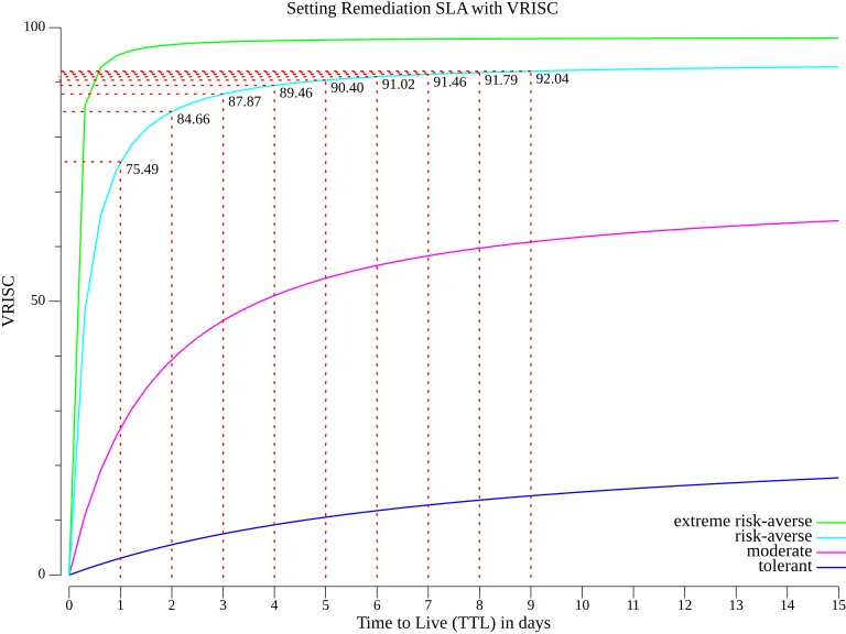
For example, suppose your organization is comfortable with a 10% Exploit Prediction Scoring System (EPSS) score (meaning a 10% chance that the vulnerability will be exploited within the next 30 days). If your tolerance for this risk is a 3-day Time to Live (TTL), you can plot VRISC (a vulnerability risk indicator) against TTL for various risk tolerances to understand how risk accumulates over time.

VRISC SLA

Taking a risk-averse posture (with a scaling factor $n = \frac{1}{3}$ in the formula $\kappa = nX$ , where $\kappa_T = \frac{3}{3}$ , $\kappa_P = \frac{0.1}{3}$ , and $\kappa_V = \frac{1}{3}$ for a single vulnerability), the plot of VRISC against TTL is shown in the second-steepest curve above. The key takeaway from this curve is how quickly risk accumulates, roughly:

75% of the risk accrues by the end of the first day.
85% by the second day.
88% by the third day.
89% by the fourth day.
90% by the fifth day.

This means that beyond Day 4, there’s a diminishing return in risk reduction, as the additional value of waiting to remediate is marginal. The steepest part of the curve occurs within the first 3-4 days, showing that remediating early is the most effective way to reduce risk within appetite.

For comparison, an extremely risk-averse organization (scaling factor $n=\frac{1}{9}$ ) would have an even steeper curve as shown by the steepest green curve, where most of the risk accumulates within the first two days. In such cases, an even faster remediation SLA is required to remain within the organization’s risk appetite.

This is how VRISC can guide the choice of remediation SLAs based on your organization’s risk appetite: by showing how quickly risk accumulates, you can prioritize early remediation to maximize risk reduction and align with your tolerance levels.

Objective 2: Reduce VRISC over time

Another use of VRISC is to track how your organization manages risk over time. Since VRISC is an indicator of how vulnerabilities drive the potential for exploit in our environment and the effect and interplay of our vulnerability-generating processes vs those that remove them, we want VRISC to trend down over time.

Process Performance Metrics

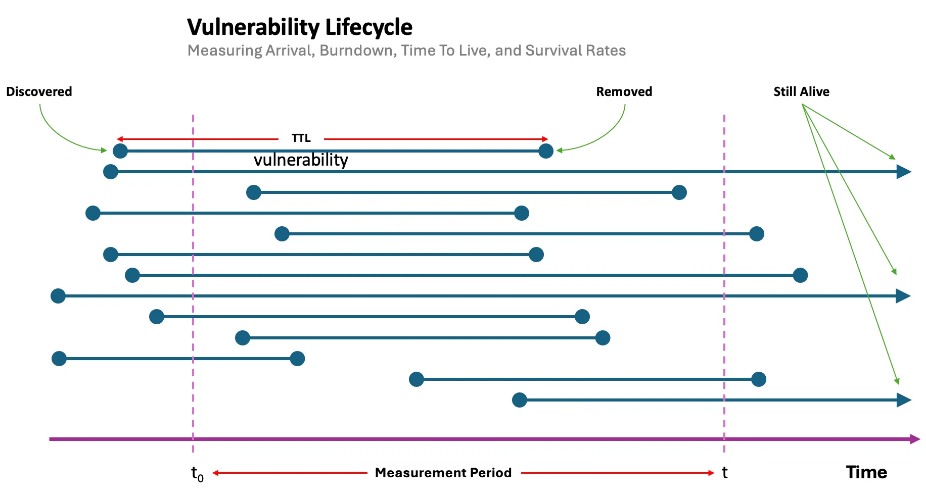
We consider other metrics that measure the performance of our vulnerability and consequently risk management processes, such as vulnerability arrival rates, burndown rates, time to live, and survival rates.

Metric	Description	Intervention points
Arrival Rate	Measures the rate at which new vulnerabilities are introduced into our environment	High arrival rates indicate weaknesses in our left of BOOM or shift left processes, and may suggest the need for interventions in processes that manage defect escape. It could also be caused by the growth of our environment, increasing your attack surface; or due to the introduction of a new vulnerability detective control, which may require that we ramp up of our triage and remediation capacity.
Burndown rate	Measures how quickly vulnerabilities are removed	This right of BOOM metric captures our process capacity to deal with forward predictors of risk. Depending on the direction of travel of other metrics such as vulnerability count growth or longer TTL and survival rates, our process capacity may be slowing, scaling or accelerating.
Time to live (TTL)	TTL is the time between the discovery and the removal of a vulnerability from the system	TTL is a measure of how long our system is exposed to the likelihood of risk materialization through the exploit of a vulnerability. The longer this window of exploit possibility, the higher our risk, as the VRISC model demonstrates.
Survival rates	Captures how long risk survives in the environment	The durability of vulnerability in our system is both an indicator or risk, and a metric that can indicate how well our processes conform to risk tolerances. For example, an survival analyses can tell us how well our system complies with a KPI that stipulates a 95% compliance with a 3-day SLA for the removal of a critical vulnerabilities.

Mathematical Definitions for the Metrics

click to open/close

vulnerability metrics

Let $V$ be the set of all vulnerabilities in the system, and let $t_0$ and $t$ be the time window for measurements, where $t_0 < t$ . The set of vulnerabilities closed within the time window, $V^\omega_{t_0,t}$ is defined as

V^\omega_{t_0,t} =\left\{ v \in V | t_0 \le v_\omega \le t \right\}

Where $v_w$ is the time vulnerability $v$ was removed (e.g. through patching).

Burndown Rate

The Burndown Rate at time $t$ , $\mu_t$ , is now defined as

\mu_t = \dfrac{|V^\omega_{t_0,t}|}{t-t_0}

Arrival Rate

Similarly, if $v_\alpha$ is the discovery time of vulnerability $v$ , then the arrival rate at time $t$ , $\lambda_t$ , is defined as

\lambda_t = \dfrac{|V^\alpha_{t_0,t}|}{t-t_0}

where

V^\alpha_{t_0,t} =\left\{ v \in V | t_0 \le v_\alpha \le t \right\}

Total Number of Open Vulnerabilities

The total number of open vulnerabilities at the time $t$ , $V_t$ is defined as follows

V_{t} = V_{t_0} + (\lambda_{t_0} - \mu_{t_0})(t- t_0)

Time to live

For vulnerability $v$ , its time to live $\text{TTL}_v$ is defined as

\text{TTL}_v = v_\omega - v_\alpha

Survival Rate

The survival rate of vulnerabilities over the time span $t_0$ and $t$ , $\psi_{t_0,t}$ , is defined as

\psi_{t_0,t} = \dfrac{|V^\psi_{t}|}{t-t_0}

where

V^\psi_{t} = \left\{ v \in V | v_\omega > t \right\}

Measuring VRISC and Other Performance Metrics Through Your Vulnerability Management Programs

Let us illustrate how you could measure your VRISC using data from your system environment and vulnerability management programs. These might include your internal vulnerability scanning or discovery tool, an external active continuous attack surface monitoring service and/or an external passive security posture monitoring solution. These all report vulnerabilities associated with your internal and external attack surfaces.

Vulnerability Data Sources

At this point, we are not focused on which part of our environment the vulnerability exists (whether externally-facing or not), or how we discovered the vulnerabilities, because our intention is to simply measure a leading indicator of risk through the growth or otherwise of vulnerabilities in our system environment.

Below are some places where you can get vulnerability data for your analysis from.

Vulnerability Discovery Sources

Consider the following sources of data to track various vulnerability-generating processes

Source	Description
Vulnerability Scanner	General vulnerabilities, CIS hardening posture benchmarks
Cloud-Native App Protection (CNAPP)	Vulnerabilities and posture/misconfigurations from Posture management (CSPM), Identity & Entitlement (CIEM), Infra as Code (IaC), Workload protection (CWP)
Continuous Attack Surface Management (CASM)	Threat intelligence-led continuous active external attack surface monitoring.
Security Rating Services	Threat intelligence-based and sinkhole data aggregating passive security posture monitoring.
SaaS Security Posture Management (SSPM)	Discovers vulnerabilities and misconfigurations in SaaS applications.
SAST, DAST, SCA	Static, Dynamic security scanning tools and Software Composition Analysis tools can discover vulnerabilities in applications, libraries and software dependencies.
Penetration Testing and Bug Bounty Program	Can discover vulnerabilities in applications and infrastructure.

Uncertainty and Data-Driven Bayesian Updating

We take a forward-looking, predictive approach to the estimation of our VRISC indicator, starting with an estimate of the factors that go into its calculation, but with the ability to adjust the estimates (through Bayesian update techniques) with data telemetry from our environment once the data becomes available. Let us illustrate the process in the next few sections.

Calculating VRISC From Vulnerability Metrics

The following approach is data-driven, but we will typically start from a point where we may not yet have data, and we have to estimate. This is absolutely fine, and our estimates do not have to be precise, since we will be using Bayesian techniques to update them once we have data from our vulnerability management process, which will improve the accuracy of our predictions over time as we get more data telemetry from the environment.

Suppose, based on our subject matter expert (SME) knowledge of our vulnerability management process, we estimate with some confidence that, on average, it takes 25 days to fix a newly discovered vulnerability, and that five new ones are discovered every week and we fix vulnerabilities at the rate of two per week. We also estimate that the probability of exploiting the discovered vulnerability is about 2% on average.

These are all estimates with a certain level of confidence associated. This is shown in the table below.

Data collection cadence

You should select a data collection period that works for your organization, for example, four weeks, which roughly lines up with the 30-day prediction period of EPSS; but the methodology works for shorter or longer reporting cadence.

Note that our estimates do not have to be precise, since we will be using Bayesian techniques to update them once we have data from our vulnerability management process, which will improve the accuracy of our predictions over time as we get more telemetry from the environment.

We provide appropriate distributions for the analysis. A little more on the distributions later.

Vulnerability Metric	Example Estimate	Probability Distribution	Conjugate Prior
TTL	25 days on average	Gamma	Gamma
Survival Rate	70 over four weeks	Beta	Beta
Arrival Rate	5 vulnerabilities per week	Poisson	Gamma
Burndown Rate	2 vulnerabilities per week	Poisson	Gamma
Vulnerability Count	800	Poisson	Gamma
Exploit Prediction Probability	2% on average per vulnerability	Binomial	Beta

Incorporating uncertainty in estimates

click to open/close

We indicate the level of uncertainty/confidence in the SME estimate by using a confidence parameter as follows:

Confidence	Description
Confident (90%)	Uncertainty, $\Delta=10\%$ , i.e. actual value lies within $\plusmn 10\%$ of the estimate
Somewhat Confident (70%)	Uncertainty, $\Delta=30\%$ , i.e. actual value lies within $\plusmn 30\%$ of the estimate
Educated Guess (50%)	Uncertainty, $\Delta=50\%$ , i.e. actual value lies within $\plusmn 50\%$ of the estimate

Let the uncertainty that we have about our SME estimate be $\Delta$ . Note that the uncertainty $\Delta > 0$ , and you should doubt anyone who claims 0% uncertainty! Incorporate the uncertainty in the analysis by defining the SME estimate as the mean $\mu$ of a distribution whose standard deviation ( $\sigma$ ) is defined as :

\begin{align} \sigma & = \Delta\mu \end{align}

Deriving starting prior Gamma distribution parameters

We have the following definitions for the starting prior Gamma distribution

\begin{align} \mu & = \dfrac{\alpha}{\beta} & \text{\small Mean of Gamma distribution (SME estimate)} \nonumber \\ \sigma^2 & = \dfrac{\alpha}{\beta^2} & \text{\small Variance of Gamma distribution} \nonumber\\ \end{align}

Substituting (1) allows us to derive the starting prior Gamma shape parameters of $\alpha$ and $\beta$ as

\begin{align} \alpha & = \dfrac{1}{\Delta^2} & \beta & = \dfrac{1}{\mu \Delta^2}\\ \end{align}

Deriving starting prior Beta distribution parameters

We have the following definitions for the starting prior Beta distribution

\begin{align} \mu & = \dfrac{\alpha}{\alpha + \beta} & \text{\small Mean of Beta distribution (SME estimate)} \nonumber \\ \sigma^2 & = \dfrac{\alpha\beta}{(\alpha+\beta)^2(\alpha+\beta+1)} & \text{\small Variance of Beta distribution} \nonumber\\ \end{align}

Substituting (1) allows us to derive the starting prior Beta shape parameters of $\alpha$ and $\beta$ as

\begin{align} \alpha & = \dfrac{1-\mu(\Delta^2 +1)}{\Delta^2} & \beta = \dfrac{\alpha(1-\mu)}{\mu} \end{align}

TBC …

Foundational Metrics and Key Risk Indicators:

Supercharge your predictive risk insight with data-driven metrics and risk indicators. (Work-in-Progress)

A Vulnerability Risk Indicator (VRISC)

Risk Aversion and Tolerance factor

Using VRISC to Set Remediation SLAs Based on Risk Tolerance

Objective 2: Reduce VRISC over time

Process Performance Metrics

Burndown Rate

Arrival Rate

Total Number of Open Vulnerabilities

Time to live

Survival Rate

Measuring VRISC and Other Performance Metrics Through Your Vulnerability Management Programs

Vulnerability Data Sources

Uncertainty and Data-Driven Bayesian Updating

Calculating VRISC From Vulnerability Metrics

Deriving starting prior Gamma distribution parameters

Deriving starting prior Beta distribution parameters

Related Posts

The Great Security Bluff: Why Your Controls Might Fail When You Need Them Most

Thriving in the VUCAH Landscape: Advanced Risk Management Strategies for CISOs

Unlocking Strategic Insights: Elevating Business Decisions with Advanced Risk Modeling

Reimagining Human Risk: How to Measure and Manage it.